Overview and Intuitive Understanding

Hidden Markov Model (HMM) is a class of probabilistic models used to model and infer system evolution processes in situations where “states are unobservable”. The core problem it solves can be summarized in one sentence:

When the true state of the real world cannot be directly observed, can we still infer the most likely internal state change process of the system based solely on the observed phenomena?

To understand this, we can start with a classic and intuitive thought experiment.

Suppose you are locked in a completely enclosed room and can never see the weather conditions outside. The real weather outside each day can only be one of three types: sunny, cloudy, or rainy. However, the only information you can get each day is that someone hands you a note recording how many ice creams a certain person ate that day.

Your goal is not to care about the ice cream itself, but to infer the most likely weather situation outside each day based on this string of “ice cream quantity” records, and even further infer how the weather changes over time.

This is exactly the typical problem structure characterized by HMM.

In this story, weather is real but cannot be directly observed, while ice cream quantity is the only external phenomenon you can see. The modeling idea of HMM is precisely to characterize the statistical relationship between these two layers of information to complete the inference process of “deducing essence from phenomena.”

Three-Element Structure of HMM

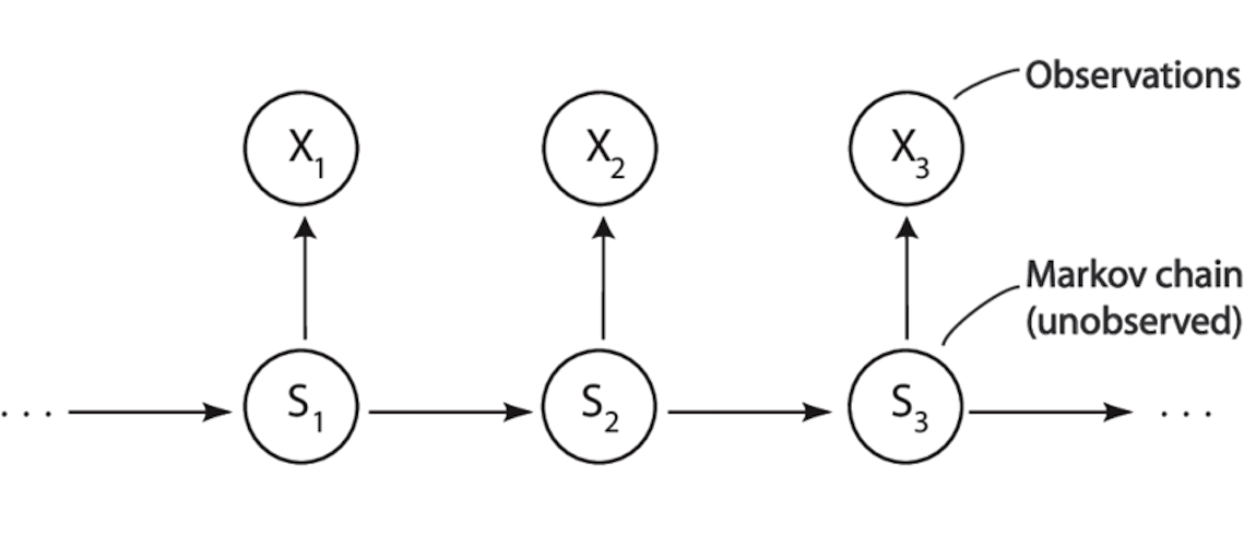
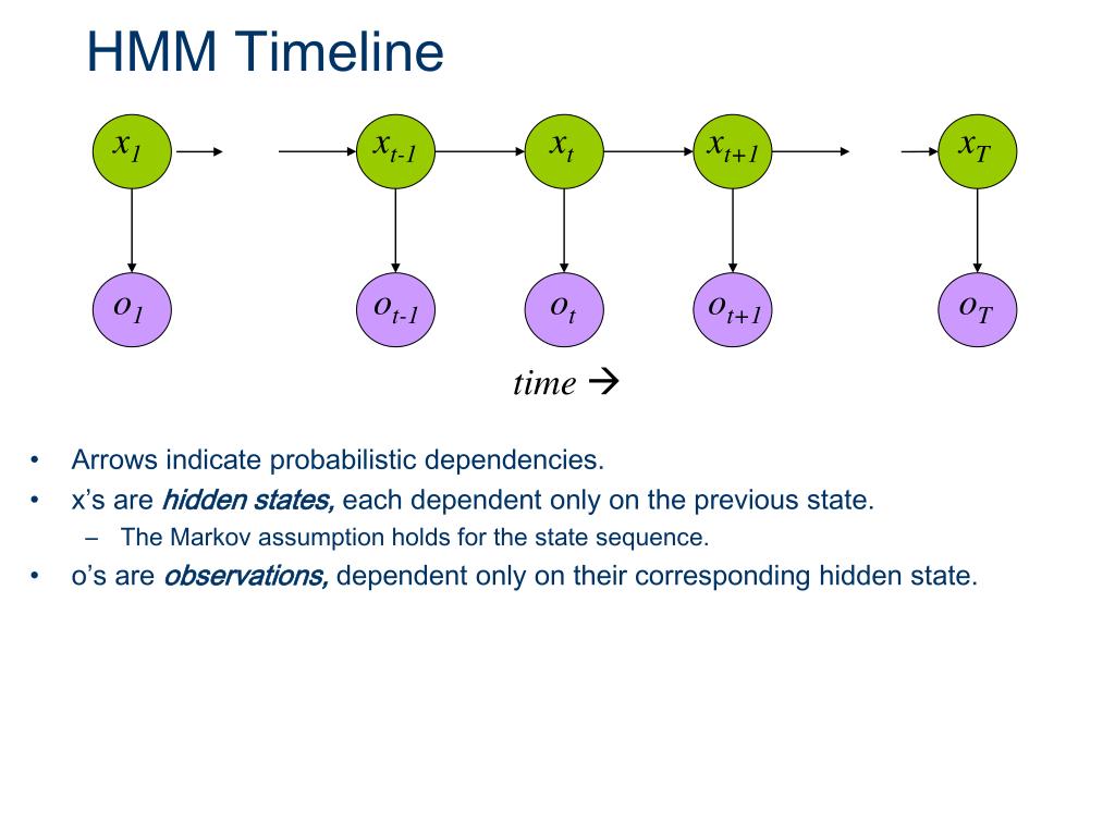
A standard HMM consists of three types of core elements: hidden states, observations, and the probability rules between them.

1. Hidden States

Hidden states describe the true internal state the system is in at each time point, but these states themselves cannot be directly observed.

In the weather-ice cream example, the hidden state set can be understood as:

Sunny, Cloudy, Rainy

These states have two important characteristics: First, they do indeed exist in reality and change over time; Second, they are not directly “exposed” to the observer, but can only be indirectly reflected through external behaviors or phenomena.

The modeling goal of HMM is precisely to infer this “invisible state sequence.”

2. Observations

Opposite to hidden states are observations, i.e., the data that observers can directly obtain at each time point.

In this example, the observation is the number of ice creams eaten each day, such as:

0, 1, 2

Observations themselves are not the ultimate object of our concern, but there is a statistical correlation between them and hidden states. It is precisely this correlation that makes “inferring states from observations” possible.

3. Probability Rules: How States Evolve, How Phenomena Are Generated

HMM does not try to describe the world through deterministic rules, but characterizes uncertainty through probability. This set of probability rules contains only two types.

The first type is state transition probability, used to describe how hidden states evolve over time. For example: If today is sunny, what is the probability that tomorrow will still be sunny? What is the probability of becoming rainy?

This assumption reflects an important fact: state changes in the real world usually have continuity and inertia, rather than completely randomly jumping. This is precisely the core meaning of “Markov property” — the future only depends on the current state and is independent of more distant history.

The second type is emission probability (observation probability), used to describe the likelihood of observing a specific observation value under a certain hidden state. For example: On a sunny day, people are more likely to eat more ice cream; on a rainy day, the probability of eating ice cream is significantly reduced.

Hidden states will not directly tell you “who I am”; they only “indirectly leave traces” through observations. HMM precisely connects invisible states with visible phenomena through this set of probability bridges.

Three Core Types of Problems HMM Needs to Solve

After clarifying the basic structure of HMM (hidden states, observation variables, transition probabilities, emission probabilities, etc.), the core problem next is not “what the model looks like,” but:

Based on this model, what inferences can we actually make?

Almost all practical applications of HMM — whether speech recognition, sequence labeling, or time series modeling — can ultimately be reduced to three essentially different but closely related types of problems. The entire algorithm system of HMM is precisely built around these three types of problems.

First Type of Problem: Given the Model, What Is the Probability of the Observation Sequence?

The first type of problem can be stated as:

Given that model parameters are completely known, what is the probability that an observation sequence appears?

In mathematical language, this means calculating for a given observation sequence

\[ O = (o_1, o_2, \dots, o_T) \]

under known model parameters

\[ \lambda = (\pi, A, B) \]

the probability:

\[ P(O \mid \lambda) \]

Why Is This Problem Important?

At first glance, this problem seems somewhat “passive,” just calculating a probability value, but it is actually the foundation of all other inference problems:

• In speech recognition, it can be used to judge “whether this model can explain the currently input speech well”;
• In model comparison, it can serve as a scoring function to judge which of multiple models is more reasonable;
• In parameter learning (the third type of problem), it is the optimization objective function itself.

Where Is the Difficulty?

If calculated directly by brute force, you need to enumerate all possible hidden state sequences:

\[ Q = (q_1, q_2, \dots, q_T) \]

The number of hidden states usually grows exponentially. This means that even if the model structure is very simple, direct enumeration is almost infeasible.

Corresponding Algorithm

To solve this “seemingly simple but computationally extremely expensive” problem, the Forward Algorithm was introduced.

Its core idea is: Through dynamic programming, transform the problem of “summing over all paths” into step-by-step recursive calculation.

The forward algorithm does not care about “which path is best”; it does only one thing:

Reasonably and efficiently add up the probabilities of all possible paths.

Second Type of Problem: Given the Observation Sequence, What Is the Most Likely Hidden State Path?

The focus of the second type of problem has changed:

Given that the observation sequence is already given, which hidden state sequence is most likely to have generated these observations?

Mathematically, this is equivalent to solving:

\[ \arg\max_Q P(Q \mid O, \lambda) \]

Intuitively, this means:

“Since these phenomena have already occurred, what should be the most reasonable ‘state evolution process’ behind the scenes?”

What Does This Problem Mean in Practice?

This type of problem is the truly concerned output result in many applications:

• In part-of-speech tagging, it corresponds to “the most likely part of speech for each word”;
• In speech recognition, it corresponds to “the most likely phoneme or state sequence”;
• In behavior modeling, it corresponds to “the internal state the system is most likely in at each moment.”

Essential Difference from the First Type of Problem

• The first type of problem is summing over all paths;
• The second type of problem is finding the maximum among all paths.

These two seem similar but are completely different tasks in computational logic.

Corresponding Algorithm

To solve the “find optimal path” problem, the Viterbi Algorithm was introduced.

It also uses dynamic programming, but the core operation is no longer “addition” but “taking maximum”:

• At each step, only keep the optimal path to reach each state at the current moment;
• By recording backtracking pointers, finally restore the entire optimal state sequence.

It can be understood as: Finding a path with maximum weight in a probability graph unfolded over time.

Third Type of Problem: Model Parameters Unknown, Can We Learn Backward from Data?

The first two types of problems both have an important premise: Model parameters are known.

But in the real world, this premise often does not hold.

Thus the third and most challenging type of problem is introduced:

When hidden states are unobservable and model parameters are unknown, can we estimate model parameters backward based solely on observation data?

In other words, given a batch of observation sequences:

\[ \{O^{(1)}, O^{(2)}, \dots, O^{(N)}\} \]

we hope to learn the most reasonable:

\[ \lambda = (\pi, A, B) \]

Why Is This Problem Difficult?

The reason lies in a “circular” dependency relationship:

• To estimate parameters, it seems we need to know hidden states;
• But hidden states are precisely what we don’t know.

In other words: We need to learn a model that describes the truth under the premise of “not seeing the truth”.

Corresponding Algorithm

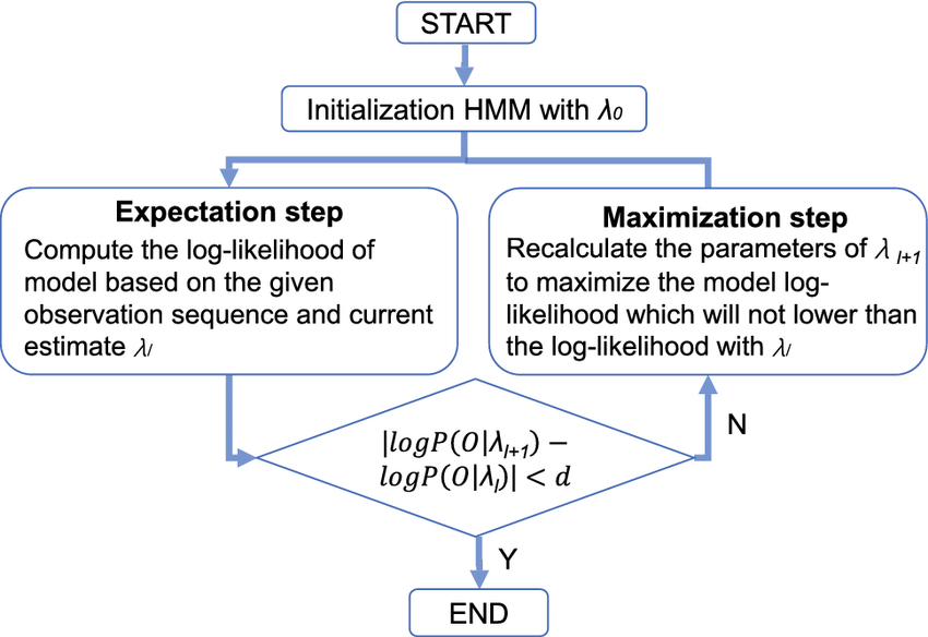
To solve this problem, the Baum–Welch Algorithm was introduced, which is essentially a special case of the EM (Expectation–Maximization) algorithm for HMM.

Its core idea can be summarized as a two-step iterative process:

1. E-step: Under current parameters, calculate “what hidden states might be” (using forward-backward algorithm);
2. M-step: Based on “expected hidden state distribution,” re-estimate model parameters.

By repeatedly iterating these two steps, model parameters will gradually converge to a local optimal solution.

Relationships Among the Three Types of Problems

These three types of problems are not isolated from each other, but progressive and interdependent:

• The forward algorithm is the basic tool for probability evaluation;
• The Viterbi algorithm is the optimal path inference tool;
• The Baum–Welch algorithm repeatedly calls forward and backward calculations internally, and is the core mechanism of parameter learning.

Understanding these three types of problems is equivalent to understanding the entire inference and learning framework of HMM.

Model Notation and Parameter Setting

Let the hidden state set be:

$$ S = \{\text{Sunny}(S), \text{Rainy}(R)\} $$

Observation set is:

$$ O = \{0, 1, 2\} $$

Initial state probability is defined as:

$$ \pi_i = P(q_1 = i) $$

State transition probability is defined as:

$$ a_{ij} = P(q_{t+1} = j \mid q_t = i) $$

Emission probability is defined as:

$$ b_j(o) = P(x_t = o \mid q_t = j) $$

A Specific HMM Example

Set the initial state distribution as:

$$ \pi_S = 0.6,\quad \pi_R = 0.4 $$

State transition matrix is:

$$ A = \begin{bmatrix} 0.7 & 0.3 \\ 0.4 & 0.6 \end{bmatrix} $$

This indicates that weather has a certain stability, but there is still a possibility of transition.

Emission probabilities are as follows:

Sunny:

$$ b_S(0)=0.1,\quad b_S(1)=0.4,\quad b_S(2)=0.5 $$

Rainy:

$$ b_R(0)=0.6,\quad b_R(1)=0.3,\quad b_R(2)=0.1 $$

Observation Sequence

Suppose the number of ice creams observed over three consecutive days is:

$$ x_{1:3} = [2, 1, 0] $$

Forward Algorithm

The goal of the forward algorithm is to calculate the probability that the entire observation sequence appears under current model parameters.

Its core idea is: although hidden states are invisible, we can probabilistically accumulate all possible state paths. To avoid exponential-level enumeration of paths, the forward algorithm uses dynamic programming for recursive calculation.

Define forward variable:

$$ \alpha_t(i) = P(x_{1:t}, q_t = i) $$

It represents the joint probability that at the end of day \(t\), all data for the first \(t\) days are observed and the system is in state \(i\).

Initialization phase:

$$ \alpha_1(i) = \pi_i \cdot b_i(x_1) $$

Substituting values gives:

$$ \alpha_1(S) = 0.30,\quad \alpha_1(R) = 0.04 $$

Recursive formula is:

$$ \alpha_t(j) = \left( \sum_i \alpha_{t-1}(i)\cdot a_{ij} \right) \cdot b_j(x_t) $$

Calculation results are:

$$ \alpha_2(S)=0.0904,\quad \alpha_2(R)=0.0342 $$ $$ \alpha_3(S)=0.007696,\quad \alpha_3(R)=0.028584 $$

Final probability of observation sequence:

$$ P(x_{1:3}) = 0.03628 $$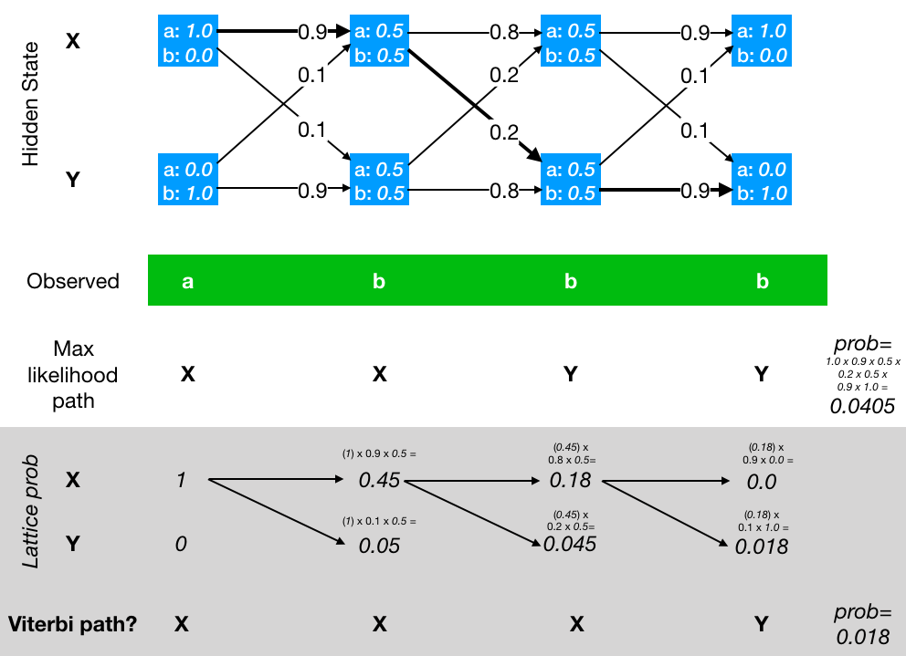

Viterbi Algorithm

Unlike the forward algorithm which sums over all paths, the Viterbi algorithm focuses on which hidden state path is most likely.

Define optimal path probability:

$$ \delta_t(j) = \max P(q_{1:t-1}, q_t = j, x_{1:t}) $$

And introduce backtracking pointer:

$$ \psi_t(j) = \arg\max \left( \delta_{t-1}(i)\cdot a_{ij} \right) $$

The optimal state path obtained by final backtracking is:

$$ [S, S, R] $$

This is highly consistent with intuition: the first two days ate more, more consistent with sunny days; the last day ate almost no ice cream, more consistent with rainy days.

Baum–Welch (EM Training Algorithm)

When model parameters are unknown, these parameters can be automatically estimated from observation data through the Baum–Welch algorithm. This algorithm is a specific implementation of the EM framework for HMM.

Its core idea is to alternately perform two steps:

E-step, estimate the probability of belonging to each hidden state at each time point under the current model; M-step, use these “soft statistical results” to re-update model parameters.

Backward variable is defined as:

$$ \beta_t(i) = P(x_{t+1:T} \mid q_t = i) $$

State posterior probability is:

$$ \gamma_t(i) = \frac{\alpha_t(i)\beta_t(i)} {\sum_k \alpha_t(k)\beta_t(k)} $$

Parameter update formulas are as follows:

$$ \pi_i \leftarrow \gamma_1(i) $$ $$ a_{ij} \leftarrow \frac{\sum_{t=1}^{T-1} \xi_t(i,j)} {\sum_{t=1}^{T-1} \gamma_t(i)} $$ $$ b_j(o) \leftarrow \frac{\sum_{t: x_t=o} \gamma_t(j)} {\sum_{t=1}^{T} \gamma_t(j)} $$

Summary

From an overall perspective, the Hidden Markov Model is not constituted by a single “isolated algorithm,” but forms a set of mutually cooperating, logically closed algorithm systems around the core goal of “how to make inferences in an unobservable world.”

The forward algorithm solves the probability evaluation problem. Under the premise that model parameters are known, it answers: “How strong is the current model’s ability to explain this observation data?” This problem itself does not directly give path or decision results, but provides the most basic quantitative basis for model comparison, model selection, and parameter learning. It can be said that the forward algorithm defines “what it means for a model to be reasonable in a probabilistic sense.”

The Viterbi algorithm focuses on the structural interpretation problem. Under the established fact that the observation sequence has already occurred, it no longer cares about the overall probability of all possibilities, but tries to give the most representative hidden state evolution path. It provides a “single-path level interpretation,” enabling HMM to answer not only “how likely” but also “how it most likely happened.”

The Baum–Welch algorithm further advances the perspective from “inference” to “learning.” Under realistic conditions where hidden states are completely unobservable, it repeatedly estimates the expected distribution of hidden states and updates model parameters accordingly, enabling HMM to complete self-adjustment and optimization relying solely on observation data. This process transforms the model from static assumptions to a dynamic system that can continuously correct itself with data.

From a logical relationship perspective, these three types of algorithms do not exist in parallel, but are progressive and interdependent: Forward (and backward) algorithms provide probabilistic characterization of hidden state uncertainty; Viterbi algorithm gives the optimal interpretation path based on this; Baum–Welch algorithm repeatedly calls probability evaluation results to achieve parameter-level learning.

It is precisely the synergistic effect of these three that makes the Hidden Markov Model not only “formally complete,” but also forms a self-consistent and operable unified framework at the three levels of inference, interpretation, and learning.